Hi,
I'ld suggest to read Section 3 of this
paper.
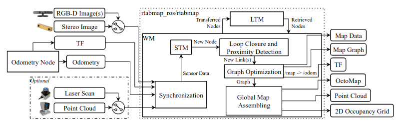
You have most parts right, though not exactly that sequence. As shown in the figure above, the occupancy grid is updated as the last step.
Basically:
1- (STM) Extract visual features, quantization of them to visual dictionary (visual words)
2- With the visual words, do BOW and try to find a global loop closure, if the hypothesis is high enough, estimate first with visual correspondences, then if icp is enabled and lidar is provided, do an icp refinement on the resulting loop closure.
3- Do proximity detection (local loop closure) based on current odometry pose. We do one proximity detection using visual features and the "closest" node in the graph, if a transform can be computed, add a proximity link. The proximity link can be refined by icp if lidar is provided. As a second step in proximity detection, if a lidar is used, we can do a pure local scan matching against close nodes in the graph, adding other proximity links if accepted.
4- Optimize the graph with the new constraints
5- Update the occupancy grid based on the updated graph.

